Lab 0: Hello R; hi git.

This lab will introduce you to the course computing workflow. The main goal is to get you setup with git in GitHub, link GitHub with RStudio and play around with a few basics.

Important

This lab will not be graded.

Note

Git is a version control system (like “Track Changes” features from Microsoft Word but more powerful) and GitHub is the home for your git-based projects on the internet (like DropBox but much better).

By the end of the lab, you will…

• Be familiar with the workflow using R, RStudio, Git, and GitHub
• Gain practice writing a reproducible report using Quarto
• Practice version control using GitHub

Getting started

Important

Your lab TA will lead you through the Getting Started section.

Log in to RStudio

• Go to https://cmgr.oit.duke.edu/containers and login with your Duke NetID and Password.
• Click STA323 to log into the Docker container. You should now see the RStudio environment.

Warning

If you haven’t yet done so, you will need to reserve a container for STA323 first.

Set up your SSH key

You will authenticate GitHub using SSH. Below are an outline of the authentication steps; you are encouraged to follow along as your TA demonstrates the steps.

Note

You only need to do this authentication process one time on a single system.

• Type credentials::ssh_setup_github() into your console.
• R will ask “No SSH key found. Generate one now?” You should click 1 for yes.
• You will generate a key. It will begin with “ssh-rsa….” R will then ask “Would you like to open a browser now?” You should click 1 for yes.
• You may be asked to provide your GitHub username and password to log into GitHub. After entering this information, you should paste the key in and give it a name. You might name it in a way that indicates where the key will be used, e.g., sta323).

You can find more detailed instructions here if you’re interested.

Configure Git

There is one more thing we need to do before getting started on the assignment. Specifically, we need to configure your git so that RStudio can communicate with GitHub. This requires two pieces of information: your name and email address.

To do so, you will use the use_git_config() function from the usethis package. (And we also need to install a package called gert just for this step.)

Type the following lines of code in the console in RStudio filling in your name and the email address associated with your GitHub account.

devtools::install_github("r-lib/gert")

usethis::use_git_config(
  user.name = "Your name", 
  user.email = "Email associated with your GitHub account"
  )

For example, mine would be

devtools::install_github("r-lib/gert")

usethis::use_git_config(
  user.name = "Alexander Fisher", 
  user.email = "alexander.fisher@duke.edu"
  )

You are now ready interact with GitHub via RStudio!

Clone the repo & start new RStudio project

• Go to the course organization at github.com/sta323-sp23 organization on GitHub. Click on the repo with the prefix lab-0. It contains the starter documents you need to complete the lab.

• Click on the green CODE button, select Use SSH (this might already be selected by default, and if it is, you’ll see the text Clone with SSH). Click on the clipboard icon to copy the repo URL.

• In RStudio, go to Project in the upper-right. Click New Project -> Version Control -> Git and paste the SSH URL under “Repository URL”. Select Create Project.

• The R Project will open by default. In the future, you can open the project manually by clicking in the upper right, Open Project, and navigate to lab-0.Rproj from the drop-down menu.

• Click lab-0.qmd to open the template Quarto file. This is where you will write up your code and narrative for the lab.

R and R Studio

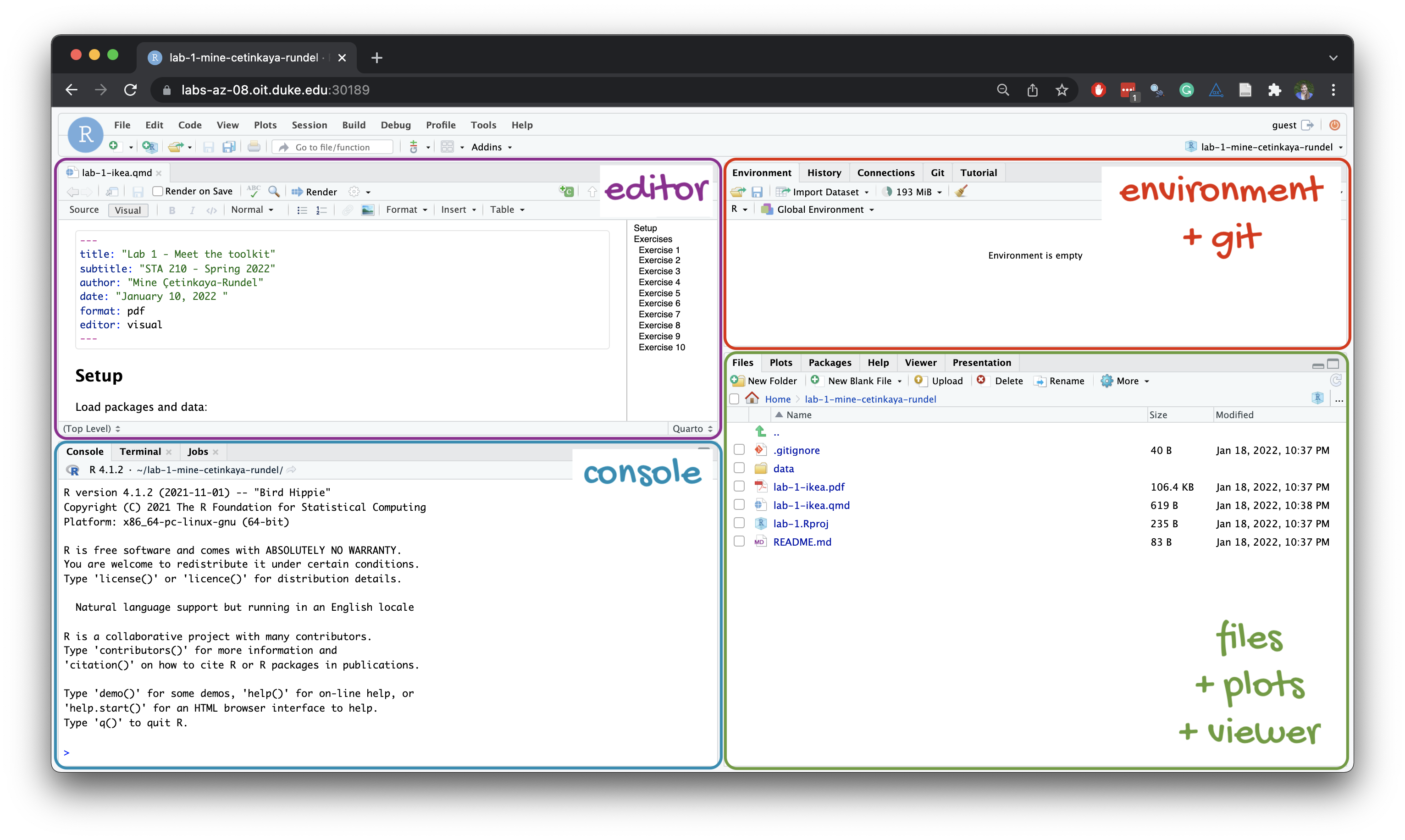
Below are the components of the RStudio IDE.

Below are the components of a Quarto (.qmd) file.

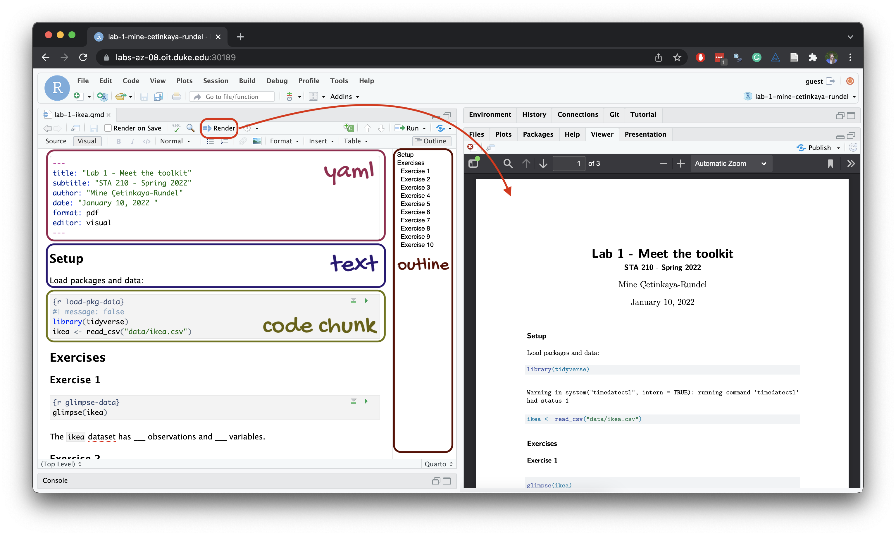
YAML

The top portion of your R Markdown file (between the three dashed lines) is called YAML. It stands for “YAML Ain’t Markup Language”. It is a human friendly data serialization standard for all programming languages. All you need to know is that this area is called the YAML (we will refer to it as such) and that it contains meta information about your document.

Important

Open the Quarto (.qmd) file in your project, change the author name to your name, and render the document. Examine the rendered document.

Committing changes

• In the Terminal pane of RStudio, type pwd to “print working directory”, i.e. show where in the filesystem you are. You should see something like /home/guest/lab-0-username. Next type ls to list files in the directory. You should see something similar:

lab-0.Rproj  README.md lab-0.qmd

• Type git status and press enter. You should see which files have been edited (highlighted in red). lab-0.qmd should be in red since you updated the YAML.

• Type git add lab-0.qmd. This stages the file to be committed. In the future you can add several files to the same commit by repeating this step. You can type git status again to see the staged file (in green). Next type git commit -m "updating YAML". This will commit the file with the message between quotes.

• Finally git push to push the changes to the remote repository.

• Now let’s make sure all the changes went to GitHub. Go to your GitHub repo and refresh the page. You should see your commit message next to the updated files. If you see this, all your changes are on GitHub and you’re good to go!

Exercises

For all exercises, you should respond in the space provided in the template lab-0.qmd and show all your work. This lab-0 just has a few warm-up exercises to introduce you to some computing phenomena and general ideas.

1. Floating point algebra.
   
   Do floating point numbers obey the rules of algebra? For example, one of the rules of algebra is additive association. (x + y) + z == x + (y + z). Check if this is true in R using \(x = 0.1\), \(y = 0.1\) and \(z = 1\). Explain what you find.

Additional examples of floating point pecularity are provided below.

# example 1
0.2 == 0.6 / 3
# example 2
point3 <- c(0.3, 0.4 - 0.1, 0.5 - 0.2, 0.6 - 0.3, 0.7 - 0.4)
point3
point3 == 0.3

To work around these issues, you could use all.equal() for checking the equality of two double quantities in R. What does all.equal() do?

# example 1, all.equal()
all.equal(0.2, 0.6 / 3)
# example 2, all.equal()
point3 <- c(0.3, 0.4 - 0.1, 0.5 - 0.2, 0.6 - 0.3, 0.7 - 0.4)
point3
all.equal(point3, rep(.3, length(point3)))

2. Inefficient math.
   
   You’ve collected 10 million observations in a vector called x and you summarize the mean of your observations:

set.seed(2)
n = 10000000
x = rnorm(n, 1, 10)
xbar = mean(x)

A new observation comes in new_x = 15.0.

new_x = 15
updated_x = c(x, new_x)

Although it won’t change much, you want to recompute the mean with this new data point. You could recompute the mean by re-running mean() on updated_x or you could observe that:

\[ \bar{x}_{n+1} = \frac{1}{n+1}(n \cdot\bar{x}_n + x_{n+1}) \]

Compare the time each method takes by surrounding each method with system.time({}).

# method 1
mean(updated_x)

#method 2
## program the equation above here and then time it with system.time({})

3. Inefficient code.
   
   To quantify the inefficiency of a poorly written for loop, time both the code blocks below. Experiment with different values of n. What do you observe?

# method 1
n <- 10
x <- 1
for (i in seq_len(n)) {
  x <- c(x, sqrt(x[i] * i))
}

# method 2
n <- 10
x <- rep(1, n + 1)
for (i in seq_len(n)) {
  x[i + 1] <- sqrt(x[i] * i)
}

4. Vector norms.

If \(x\) and \(y\) are scalar numbers, \(x<y\) makes sense. How do you compare the size of two different vectors \(x\) and \(y\)? A very typical way is the vector norm. The p-norm of vector \(x\) of length \(n\) is:

\[ ||x||_p = \left( \sum_{i=1}^n |x_i |^p \right)^{1/p} \]

for \(p = 1, 2, ...\). For example, if \(p = 2\) we have the Euclidean norm, also known as the \(l_2\) (read “L-2”) norm.

• Verify that the Euclidean norm of \(x = \left( 1, 2.5, -6.3 \right)\) is 6.851277 in R. You can compute the \(l_1\) and \(l_2\) norms in R using norm(x, type = "1") and norm(x, type = "2") respectively. Read the documentation, ?norm() and you will see you need to make sure the argument x is a matrix.

• Compare \(||x||_2\) and \(||y||_2\) where \(y = \left(0.8, 2.4, -6.4 \right)\).

• Compare \(||x||_1\) and \(||y||_1\), where again \(x\) and \(y\) are the vectors given above. Which is larger?

Style guidelines

All assignments in this course must employ proper coding style, as outlined below:

• All code should obey the 80 character limit per line (i.e. no code should run off the page when rendering or require scrolling). To enable a vertical line in the RStudio IDE that helps guide this, go to Tools > Global Options > Code > Display > Show margin > 80. This will enable a vertical line in your .qmd files that shows you where the 80 character cutoff is for code chunks. Instructions may vary slightly for local installs of RStudio.

• All commas should be followed by a space.

• All binary operators should be surrounded by space. For example x + y is appropriate. x+y is not.

• All pipes %>% or |> as well as ggplot layers + should be followed by a new line.

• You should be consistent with stylistic choices, e.g. only use 1 of = vs <- and %>% vs |>

• Your name should be at the top (in the YAML) of each document under “author:”

• All code chunks should be named (with names that don’t have spaces, e.g. ex-1, ex-2 etc.)

• File names in your GitHub repo such as lab-0.qmd must not be changed and left as provided.

If you have any questions about style, please ask a member of the teaching team.

Submitting your lab

For future lab assignments (this one isn’t graded), you will submit your lab assignment by simply committing and pushing your completed lab-x.qmd to your GitHub repo. Your most recent commit 48 hours after the assignment deadline will be graded, and any applicable late penalty will be applied (see the syllabus).