Tidyverse

Dr. Alexander Fisher

Duke University

Tidy data

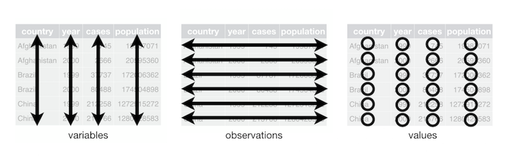
from R4DS tidy data

Tidy vs untidy

List of 3
 $ :List of 8
  ..$ name      : chr "Luke Skywalker"
  ..$ height    : chr "172"
  ..$ mass      : chr "77"
  ..$ hair_color: chr "blond"
  ..$ skin_color: chr "fair"
  ..$ eye_color : chr "blue"
  ..$ birth_year: chr "19BBY"
  ..$ gender    : chr "male"
 $ :List of 8
  ..$ name      : chr "C-3PO"
  ..$ height    : chr "167"
  ..$ mass      : chr "75"
  ..$ hair_color: chr "n/a"
  ..$ skin_color: chr "gold"
  ..$ eye_color : chr "yellow"
  ..$ birth_year: chr "112BBY"
  ..$ gender    : chr "n/a"
 $ :List of 8
  ..$ name      : chr "R2-D2"
  ..$ height    : chr "96"
  ..$ mass      : chr "32"
  ..$ hair_color: chr "n/a"
  ..$ skin_color: chr "white, blue"
  ..$ eye_color : chr "red"
  ..$ birth_year: chr "33BBY"
  ..$ gender    : chr "n/a"

untidy!

Tidy vs untidy

# A tibble: 317 × 7
   artist         track                   date.entered   wk1   wk2   wk3   wk4
   <chr>          <chr>                   <date>       <dbl> <dbl> <dbl> <dbl>
 1 2 Pac          Baby Don't Cry (Keep... 2000-02-26      87    82    72    77
 2 2Ge+her        The Hardest Part Of ... 2000-09-02      91    87    92    NA
 3 3 Doors Down   Kryptonite              2000-04-08      81    70    68    67
 4 3 Doors Down   Loser                   2000-10-21      76    76    72    69
 5 504 Boyz       Wobble Wobble           2000-04-15      57    34    25    17
 6 98^0           Give Me Just One Nig... 2000-08-19      51    39    34    26
 7 A*Teens        Dancing Queen           2000-07-08      97    97    96    95
 8 Aaliyah        I Don't Wanna           2000-01-29      84    62    51    41
 9 Aaliyah        Try Again               2000-03-18      59    53    38    28
10 Adams, Yolanda Open My Heart           2000-08-26      76    76    74    69
# … with 307 more rows

Basically tidy, but we have repeated measures.

Reshape the data

Pivot longer

library(tidyr)
table4a |>
  pivot_longer(2:3, names_to = "year", values_to = "cases")

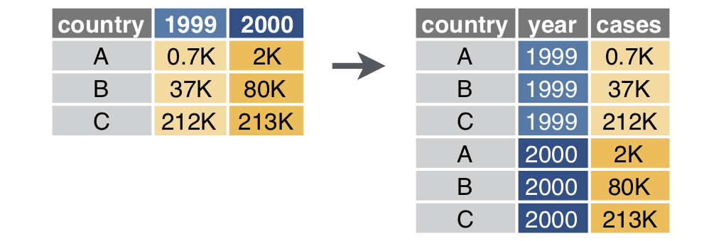
# A tibble: 6 × 3
  country     year   cases
  <chr>       <chr>  <int>
1 Afghanistan 1999     745
2 Afghanistan 2000    2666
3 Brazil      1999   37737
4 Brazil      2000   80488
5 China       1999  212258
6 China       2000  213766

From data import cheatsheet

Pivot wider

library(tidyr)
table2 |>
  pivot_wider(names_from = type, values_from = count)

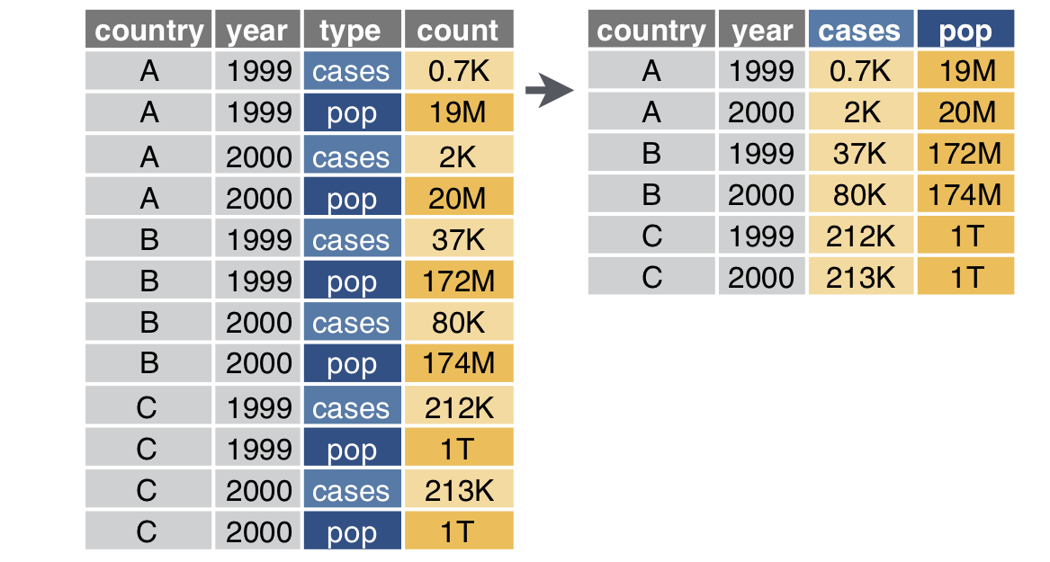
# A tibble: 6 × 4
  country      year  cases population
  <chr>       <int>  <int>      <int>
1 Afghanistan  1999    745   19987071
2 Afghanistan  2000   2666   20595360
3 Brazil       1999  37737  172006362
4 Brazil       2000  80488  174504898
5 China        1999 212258 1272915272
6 China        2000 213766 1280428583

From data import cheatsheet

Exercise 1

Reshape the billboard data set from the package tidyr so that song/week pairs make a single observation.

tidyr::billboard |>
  head(10)

# A tibble: 10 × 79
   artist track date.ent…¹   wk1   wk2   wk3   wk4   wk5   wk6   wk7   wk8   wk9
   <chr>  <chr> <date>     <dbl> <dbl> <dbl> <dbl> <dbl> <dbl> <dbl> <dbl> <dbl>
 1 2 Pac  Baby… 2000-02-26    87    82    72    77    87    94    99    NA    NA
 2 2Ge+h… The … 2000-09-02    91    87    92    NA    NA    NA    NA    NA    NA
 3 3 Doo… Kryp… 2000-04-08    81    70    68    67    66    57    54    53    51
 4 3 Doo… Loser 2000-10-21    76    76    72    69    67    65    55    59    62
 5 504 B… Wobb… 2000-04-15    57    34    25    17    17    31    36    49    53
 6 98^0   Give… 2000-08-19    51    39    34    26    26    19     2     2     3
 7 A*Tee… Danc… 2000-07-08    97    97    96    95   100    NA    NA    NA    NA
 8 Aaliy… I Do… 2000-01-29    84    62    51    41    38    35    35    38    38
 9 Aaliy… Try … 2000-03-18    59    53    38    28    21    18    16    14    12
10 Adams… Open… 2000-08-26    76    76    74    69    68    67    61    58    57
# … with 67 more variables: wk10 <dbl>, wk11 <dbl>, wk12 <dbl>, wk13 <dbl>,
#   wk14 <dbl>, wk15 <dbl>, wk16 <dbl>, wk17 <dbl>, wk18 <dbl>, wk19 <dbl>,
#   wk20 <dbl>, wk21 <dbl>, wk22 <dbl>, wk23 <dbl>, wk24 <dbl>, wk25 <dbl>,
#   wk26 <dbl>, wk27 <dbl>, wk28 <dbl>, wk29 <dbl>, wk30 <dbl>, wk31 <dbl>,
#   wk32 <dbl>, wk33 <dbl>, wk34 <dbl>, wk35 <dbl>, wk36 <dbl>, wk37 <dbl>,
#   wk38 <dbl>, wk39 <dbl>, wk40 <dbl>, wk41 <dbl>, wk42 <dbl>, wk43 <dbl>,
#   wk44 <dbl>, wk45 <dbl>, wk46 <dbl>, wk47 <dbl>, wk48 <dbl>, wk49 <dbl>, …

Pipes

A quick note on pipes

In the previous examples, you saw the base R pipe |>.

The pipe links functions and arguments together in an easy to read way.

Specifically, the pipe takes what comes before and makes it an argument to what comes after.

Example

• nested functions

park(drive(start_car(find("keys")), to = "campus"))

• pipeline

find("keys") %>%
    start_car() %>%
    drive(to = "campus") %>%
    park()

Base r vs magrittr

There are two pipes we’ll encounter in R:

• the base R pipe |> added in R v4.1.0
• the magrittr pipe %>%

The main differences are:

• the base pipe doesn’t require loading the package magrittr (contained in the tidyverse)
• the base pipe is negligibly faster in some cases
• the base pipe doesn’t support . argument passing

Example

x = c(1, 3, NA)

TRUE %>%
  mean(x, na.rm = .)

[1] 2

TRUE |>
  mean(x, na.rm = .)

Error in mean.default(TRUE, x, na.rm = .): object '.' not found

dplyr

dplyr verbs

dplyr names functions as verbs that manipulate data frames

Quick summary of key dplyr function from dplyr vignette:

Rows:

• filter():chooses rows based on column values. See logical operations
• slice(): chooses rows based on location.
• arrange(): changes the order of the rows
• distinct(): filter for unique rows (.keep_all = TRUE is useful)
• sample_n(): take a random subset of the rows

Columns:

• select(): changes whether or not a column is included.
• rename(): changes the name of columns.
• mutate(): changes the values of columns and creates new columns.
• pull(): grab column as a vector
• relocate(): change column order

Groups of rows:

• summarise(): collapses a group into a single row.
• count(): count unique values of one or more variables.
• group_by()/ungroup(): modify other verbs to act on subsets

… and more

dplyr rules

1. First argument is always a data frame

2. Subsequent arguments say what to do with that data frame

3. Always return a data frame

4. Don’t modify in place

5. Lazy evaluation magic

NYC flights

library(nycflights13)
glimpse(flights)

Rows: 336,776
Columns: 19
$ year           <int> 2013, 2013, 2013, 2013, 2013, 2013, 2013, 2013, 2013, 2…
$ month          <int> 1, 1, 1, 1, 1, 1, 1, 1, 1, 1, 1, 1, 1, 1, 1, 1, 1, 1, 1…
$ day            <int> 1, 1, 1, 1, 1, 1, 1, 1, 1, 1, 1, 1, 1, 1, 1, 1, 1, 1, 1…
$ dep_time       <int> 517, 533, 542, 544, 554, 554, 555, 557, 557, 558, 558, …
$ sched_dep_time <int> 515, 529, 540, 545, 600, 558, 600, 600, 600, 600, 600, …
$ dep_delay      <dbl> 2, 4, 2, -1, -6, -4, -5, -3, -3, -2, -2, -2, -2, -2, -1…
$ arr_time       <int> 830, 850, 923, 1004, 812, 740, 913, 709, 838, 753, 849,…
$ sched_arr_time <int> 819, 830, 850, 1022, 837, 728, 854, 723, 846, 745, 851,…
$ arr_delay      <dbl> 11, 20, 33, -18, -25, 12, 19, -14, -8, 8, -2, -3, 7, -1…
$ carrier        <chr> "UA", "UA", "AA", "B6", "DL", "UA", "B6", "EV", "B6", "…
$ flight         <int> 1545, 1714, 1141, 725, 461, 1696, 507, 5708, 79, 301, 4…
$ tailnum        <chr> "N14228", "N24211", "N619AA", "N804JB", "N668DN", "N394…
$ origin         <chr> "EWR", "LGA", "JFK", "JFK", "LGA", "EWR", "EWR", "LGA",…
$ dest           <chr> "IAH", "IAH", "MIA", "BQN", "ATL", "ORD", "FLL", "IAD",…
$ air_time       <dbl> 227, 227, 160, 183, 116, 150, 158, 53, 140, 138, 149, 1…
$ distance       <dbl> 1400, 1416, 1089, 1576, 762, 719, 1065, 229, 944, 733, …
$ hour           <dbl> 5, 5, 5, 5, 6, 5, 6, 6, 6, 6, 6, 6, 6, 6, 6, 5, 6, 6, 6…
$ minute         <dbl> 15, 29, 40, 45, 0, 58, 0, 0, 0, 0, 0, 0, 0, 0, 0, 59, 0…
$ time_hour      <dttm> 2013-01-01 05:00:00, 2013-01-01 05:00:00, 2013-01-01 0…

Examples

distinct()

How many flights are in the data set?

flights %>%
  distinct(tailnum) %>%
  nrow()

[1] 4044

How many distinct routes?

flights %>%
  select(origin, dest) %>%
  distinct() %>%
  nrow()

[1] 224

select() two columns

select(flights, arr_delay, dest)

# A tibble: 336,776 × 2
   arr_delay dest 
       <dbl> <chr>
 1        11 IAH  
 2        20 IAH  
 3        33 MIA  
 4       -18 BQN  
 5       -25 ATL  
 6        12 ORD  
 7        19 FLL  
 8       -14 IAD  
 9        -8 MCO  
10         8 ORD  
# … with 336,766 more rows

select() columns that contain information about departures or arrivals

flights %>% 
  select(contains("dep_"), contains("arr_"))

# A tibble: 336,776 × 6
   dep_time sched_dep_time dep_delay arr_time sched_arr_time arr_delay
      <int>          <int>     <dbl>    <int>          <int>     <dbl>
 1      517            515         2      830            819        11
 2      533            529         4      850            830        20
 3      542            540         2      923            850        33
 4      544            545        -1     1004           1022       -18
 5      554            600        -6      812            837       -25
 6      554            558        -4      740            728        12
 7      555            600        -5      913            854        19
 8      557            600        -3      709            723       -14
 9      557            600        -3      838            846        -8
10      558            600        -2      753            745         8
# … with 336,766 more rows

select() the numeric (or not numeric) columns

flights %>% 
  select(where(is.numeric)) %>%
  head(3)

# A tibble: 3 × 14
   year month   day dep_time sched_dep_…¹ dep_d…² arr_t…³ sched…⁴ arr_d…⁵ flight
  <int> <int> <int>    <int>        <int>   <dbl>   <int>   <int>   <dbl>  <int>
1  2013     1     1      517          515       2     830     819      11   1545
2  2013     1     1      533          529       4     850     830      20   1714
3  2013     1     1      542          540       2     923     850      33   1141
# … with 4 more variables: air_time <dbl>, distance <dbl>, hour <dbl>,
#   minute <dbl>, and abbreviated variable names ¹​sched_dep_time, ²​dep_delay,
#   ³​arr_time, ⁴​sched_arr_time, ⁵​arr_delay

flights %>% 
  select(where(function(x) !is.numeric(x))) %>%
  head(5)

# A tibble: 5 × 5
  carrier tailnum origin dest  time_hour          
  <chr>   <chr>   <chr>  <chr> <dttm>             
1 UA      N14228  EWR    IAH   2013-01-01 05:00:00
2 UA      N24211  LGA    IAH   2013-01-01 05:00:00
3 AA      N619AA  JFK    MIA   2013-01-01 05:00:00
4 B6      N804JB  JFK    BQN   2013-01-01 05:00:00
5 DL      N668DN  LGA    ATL   2013-01-01 06:00:00

exclude with select()

select() all but the first 10 columns

flights %>%
  select(-1:10)

Warning in x:y: numerical expression has 18 elements: only the first used

# A tibble: 336,776 × 9
   month   day dep_time sched_dep_time dep_delay arr_t…¹ sched…² arr_d…³ carrier
   <int> <int>    <int>          <int>     <dbl>   <int>   <int>   <dbl> <chr>  
 1     1     1      517            515         2     830     819      11 UA     
 2     1     1      533            529         4     850     830      20 UA     
 3     1     1      542            540         2     923     850      33 AA     
 4     1     1      544            545        -1    1004    1022     -18 B6     
 5     1     1      554            600        -6     812     837     -25 DL     
 6     1     1      554            558        -4     740     728      12 UA     
 7     1     1      555            600        -5     913     854      19 B6     
 8     1     1      557            600        -3     709     723     -14 EV     
 9     1     1      557            600        -3     838     846      -8 B6     
10     1     1      558            600        -2     753     745       8 AA     
# … with 336,766 more rows, and abbreviated variable names ¹​arr_time,
#   ²​sched_arr_time, ³​arr_delay

relocate()

flights %>% 
  relocate(carrier, origin, dest) %>% # to the front
  names()

 [1] "carrier"        "origin"         "dest"           "year"          
 [5] "month"          "day"            "dep_time"       "sched_dep_time"
 [9] "dep_delay"      "arr_time"       "sched_arr_time" "arr_delay"     
[13] "flight"         "tailnum"        "air_time"       "distance"      
[17] "hour"           "minute"         "time_hour"     

flights %>%
  relocate(year, month, day, .after = last_col()) %>% # to the end
  names()

 [1] "dep_time"       "sched_dep_time" "dep_delay"      "arr_time"      
 [5] "sched_arr_time" "arr_delay"      "carrier"        "flight"        
 [9] "tailnum"        "origin"         "dest"           "air_time"      
[13] "distance"       "hour"           "minute"         "time_hour"     
[17] "year"           "month"          "day"           

rename()

change the column names

flights %>% 
  relocate(tailnum) %>% 
  rename(tail_number = tailnum)

# A tibble: 336,776 × 19
   tail_number  year month   day dep_t…¹ sched…² dep_d…³ arr_t…⁴ sched…⁵ arr_d…⁶
   <chr>       <int> <int> <int>   <int>   <int>   <dbl>   <int>   <int>   <dbl>
 1 N14228       2013     1     1     517     515       2     830     819      11
 2 N24211       2013     1     1     533     529       4     850     830      20
 3 N619AA       2013     1     1     542     540       2     923     850      33
 4 N804JB       2013     1     1     544     545      -1    1004    1022     -18
 5 N668DN       2013     1     1     554     600      -6     812     837     -25
 6 N39463       2013     1     1     554     558      -4     740     728      12
 7 N516JB       2013     1     1     555     600      -5     913     854      19
 8 N829AS       2013     1     1     557     600      -3     709     723     -14
 9 N593JB       2013     1     1     557     600      -3     838     846      -8
10 N3ALAA       2013     1     1     558     600      -2     753     745       8
# … with 336,766 more rows, 9 more variables: carrier <chr>, flight <int>,
#   origin <chr>, dest <chr>, air_time <dbl>, distance <dbl>, hour <dbl>,
#   minute <dbl>, time_hour <dttm>, and abbreviated variable names ¹​dep_time,
#   ²​sched_dep_time, ³​dep_delay, ⁴​arr_time, ⁵​sched_arr_time, ⁶​arr_delay

re-name with select()

flights %>% 
  select(tail_number = tailnum)

# A tibble: 336,776 × 1
   tail_number
   <chr>      
 1 N14228     
 2 N24211     
 3 N619AA     
 4 N804JB     
 5 N668DN     
 6 N39463     
 7 N516JB     
 8 N829AS     
 9 N593JB     
10 N3ALAA     
# … with 336,766 more rows

arrange()

set.seed(10)
flights %>% 
  slice_sample(n = 3) %>% 
  select(tailnum, day) %>% 
  arrange(day)

# A tibble: 3 × 2
  tailnum   day
  <chr>   <int>
1 N258JB     17
2 N3CPAA     20
3 N515MJ     31

set.seed(10)
flights %>% 
  slice_sample(n = 3) %>% 
  select(tailnum, day) %>% 
  arrange(desc(day))

# A tibble: 3 × 2
  tailnum   day
  <chr>   <int>
1 N515MJ     31
2 N3CPAA     20
3 N258JB     17

• arrange() defaults to ascending order. Use desc() for descending order.

• you can arrange by multiple columns

group_by()

flights %>% 
  group_by(origin)

# A tibble: 336,776 × 19
# Groups:   origin [3]
    year month   day dep_time sched_de…¹ dep_d…² arr_t…³ sched…⁴ arr_d…⁵ carrier
   <int> <int> <int>    <int>      <int>   <dbl>   <int>   <int>   <dbl> <chr>  
 1  2013     1     1      517        515       2     830     819      11 UA     
 2  2013     1     1      533        529       4     850     830      20 UA     
 3  2013     1     1      542        540       2     923     850      33 AA     
 4  2013     1     1      544        545      -1    1004    1022     -18 B6     
 5  2013     1     1      554        600      -6     812     837     -25 DL     
 6  2013     1     1      554        558      -4     740     728      12 UA     
 7  2013     1     1      555        600      -5     913     854      19 B6     
 8  2013     1     1      557        600      -3     709     723     -14 EV     
 9  2013     1     1      557        600      -3     838     846      -8 B6     
10  2013     1     1      558        600      -2     753     745       8 AA     
# … with 336,766 more rows, 9 more variables: flight <int>, tailnum <chr>,
#   origin <chr>, dest <chr>, air_time <dbl>, distance <dbl>, hour <dbl>,
#   minute <dbl>, time_hour <dttm>, and abbreviated variable names
#   ¹​sched_dep_time, ²​dep_delay, ³​arr_time, ⁴​sched_arr_time, ⁵​arr_delay

summarize() with group_by()

flights %>% 
  group_by(origin) %>%
  summarize(
    n = n(), 
    min_dep_delay = min(dep_delay, na.rm = TRUE), 
    max_dep_delay = max(dep_delay, na.rm = TRUE)
  )

# A tibble: 3 × 4
  origin      n min_dep_delay max_dep_delay
  <chr>   <int>         <dbl>         <dbl>
1 EWR    120835           -25          1126
2 JFK    111279           -43          1301
3 LGA    104662           -33           911

Groups after summarize

flights %>% 
  group_by(origin) %>%
  summarize(
    n = n(), 
    min_dep_delay = min(dep_delay, na.rm = TRUE), 
    max_dep_delay = max(dep_delay, na.rm = TRUE),
    .groups = "drop_last"
  )

# A tibble: 3 × 4
  origin      n min_dep_delay max_dep_delay
  <chr>   <int>         <dbl>         <dbl>
1 EWR    120835           -25          1126
2 JFK    111279           -43          1301
3 LGA    104662           -33           911

flights %>% 
  group_by(origin) %>%
  summarize(
    n = n(), 
    min_dep_delay = min(dep_delay, na.rm = TRUE), 
    max_dep_delay = max(dep_delay, na.rm = TRUE),
    .groups = "keep"
  )

# A tibble: 3 × 4
# Groups:   origin [3]
  origin      n min_dep_delay max_dep_delay
  <chr>   <int>         <dbl>         <dbl>
1 EWR    120835           -25          1126
2 JFK    111279           -43          1301
3 LGA    104662           -33           911

count()

count() is a quick group_by() and summarize()

flights %>% 
  group_by(origin, carrier) %>%
  summarize(n = n(), .groups = "drop")

# A tibble: 35 × 3
   origin carrier     n
   <chr>  <chr>   <int>
 1 EWR    9E       1268
 2 EWR    AA       3487
 3 EWR    AS        714
 4 EWR    B6       6557
 5 EWR    DL       4342
 6 EWR    EV      43939
 7 EWR    MQ       2276
 8 EWR    OO          6
 9 EWR    UA      46087
10 EWR    US       4405
# … with 25 more rows

flights %>%
  count(origin, carrier)

# A tibble: 35 × 3
   origin carrier     n
   <chr>  <chr>   <int>
 1 EWR    9E       1268
 2 EWR    AA       3487
 3 EWR    AS        714
 4 EWR    B6       6557
 5 EWR    DL       4342
 6 EWR    EV      43939
 7 EWR    MQ       2276
 8 EWR    OO          6
 9 EWR    UA      46087
10 EWR    US       4405
# … with 25 more rows

mutate() with group_by()

flights %>% group_by(origin) %>%
  mutate(
    n = n(), 
  ) %>%
  select(origin, n)

# A tibble: 336,776 × 2
# Groups:   origin [3]
   origin      n
   <chr>   <int>
 1 EWR    120835
 2 LGA    104662
 3 JFK    111279
 4 JFK    111279
 5 LGA    104662
 6 EWR    120835
 7 EWR    120835
 8 LGA    104662
 9 JFK    111279
10 LGA    104662
# … with 336,766 more rows

combined example

What’s the average speed in miles per hour of flights traveling to Raleigh-Durham, Atlanta and Orlando airports?

flights %>% 
  filter(dest %in% c("RDU", "ATL", "MCO")) %>%
  mutate(time_hours = air_time / 60) %>%
  mutate(mph = distance / time_hours) %>%
  group_by(dest) %>%
  summarize(mean_speed = mean(mph, na.rm = TRUE))

# A tibble: 3 × 2
  dest  mean_speed
  <chr>      <dbl>
1 ATL         405.
2 MCO         422.
3 RDU         364.

Take the flights data frame and then filter for destination airports: (RDU, ATL, MCO).

Next mutate a new column time_hours that reports air time of the flight in hours.

Mutate a column mph that reports miles per hour.

Group by destination and then summarize the mean flight speed towards each destination.

Exercise 2

Using the flights data frame within the nycflights13 package:

• Which plane (check the tail number) flew out of each New York airport the most?

• Which day of the year should you fly on if you want to have the lowest possible average departure delay? What about arrival delay?

• What was the shortest flight out of each airport in terms of distance?