Importance sampling
Duke University
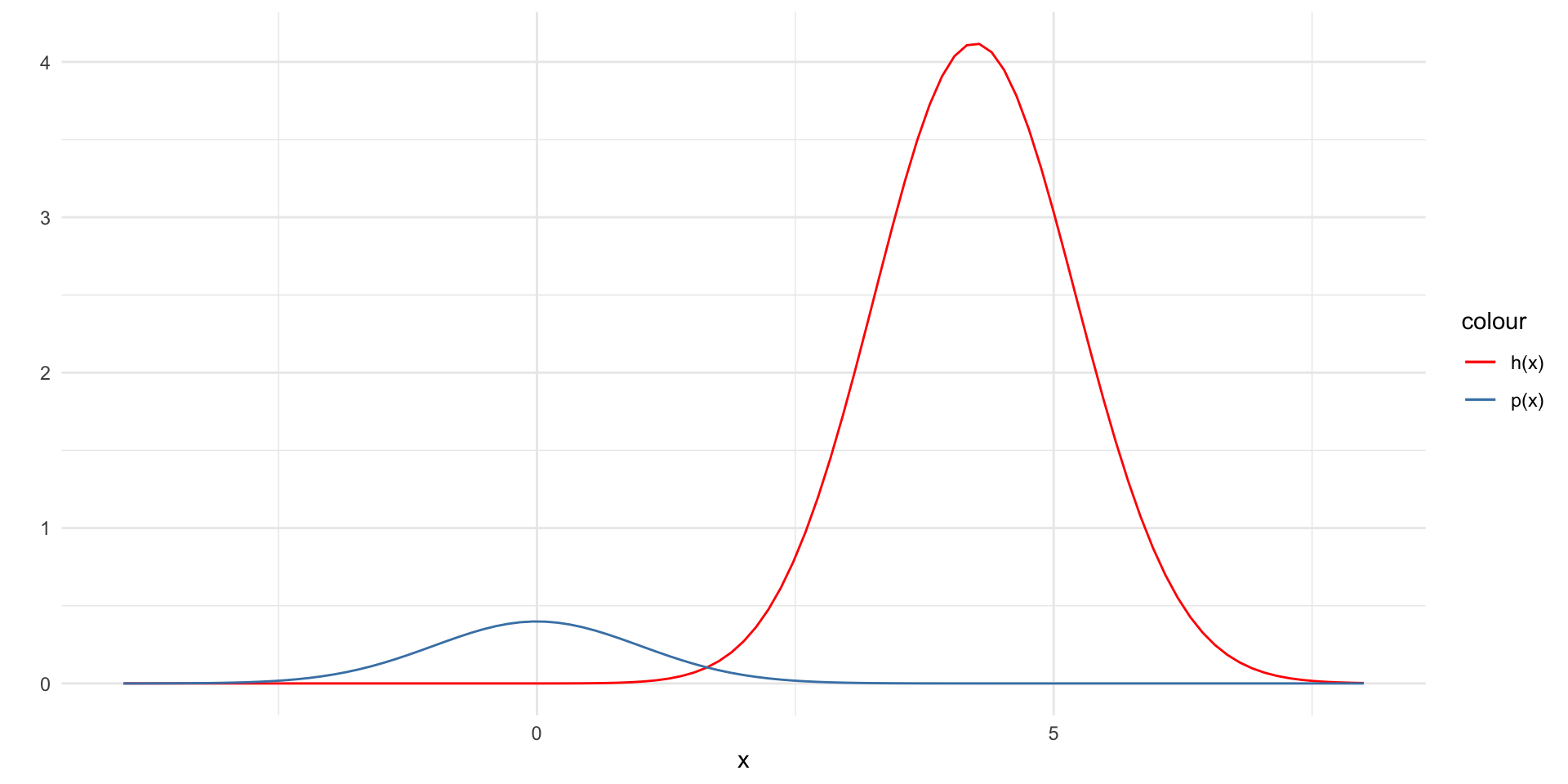
\(p(x)\) off from \(h(x)\)
- Note: here \(h(x) = x~e^{-\frac{(x-4)^2}{2}} \frac{1}{\sqrt{2\pi}}\) (i.e. I am dropping the indicator function for illustrative purposes)
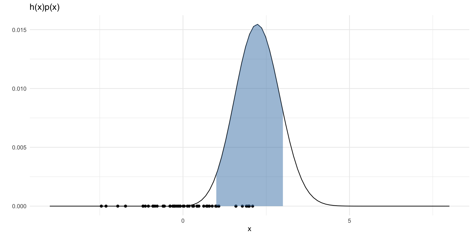
Samples not good for \(h(x)p(x)\)
set.seed(2)
hp = function(x) {
h(x) * dnorm(x)
}
N = 50
points = data.frame(x = rnorm(N, 0, 1),
y = rep(0, N))
ggplot() +
xlim(-4, 8) +
geom_function(fun = hp) +
geom_point(data = points, aes(x = x, y = y)) +
labs(x = "x", y = "") +
theme_minimal() +
labs(title = "h(x)p(x)") +
stat_function(fun = hp,
xlim = c(1,3),
geom = "area",
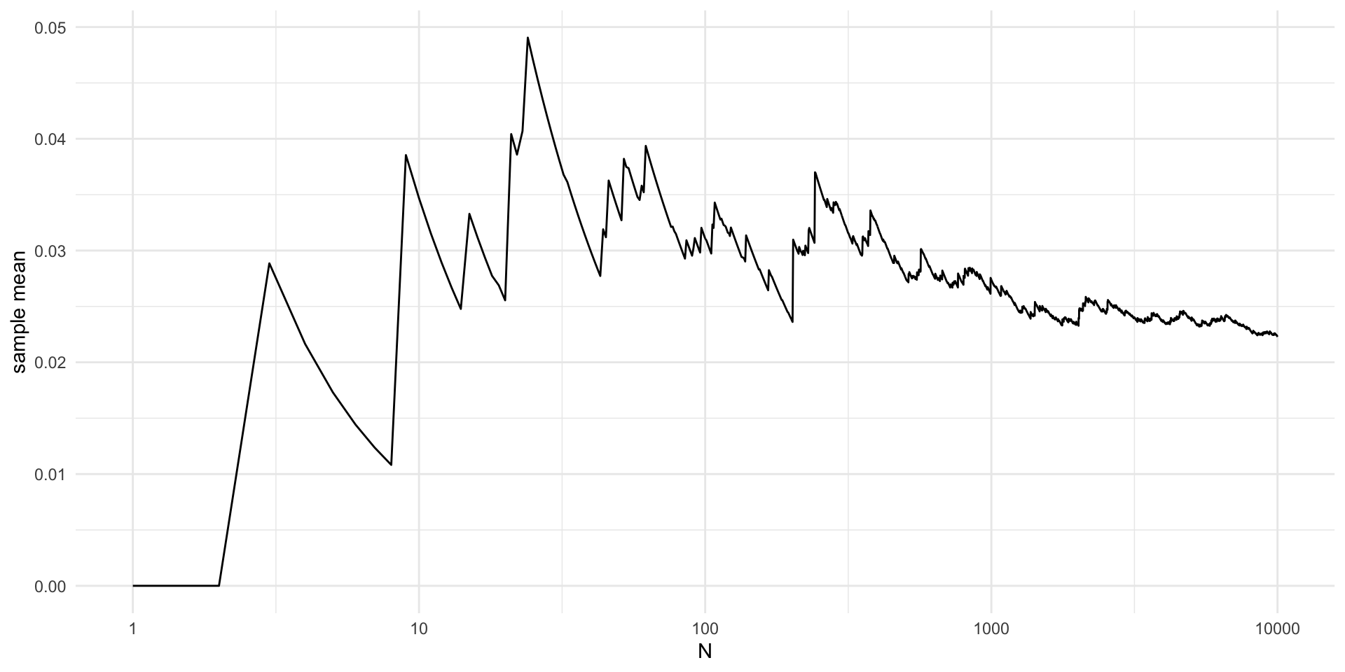
fill = "steelblue", alpha = 0.5)Resulting in large approximation error
library(magrittr)
set.seed(2)
N = 10000
x = rnorm(N, 0, 1)

h1 = function(x) {
z = h(x)
z[x < 1] = 0
z[x > 3] = 0
  return(z)
}

estimate = vector(length = N)
for (n in 1:N) {
  estimate[n] = mean(h1(x[1:n]))
}

V = data.frame(x = seq(N),
               y = estimate)

V %>%
  ggplot(aes(x = x, y = y)) +
  geom_line() +
  theme_minimal() +
  labs(x = "N", y = "sample mean") +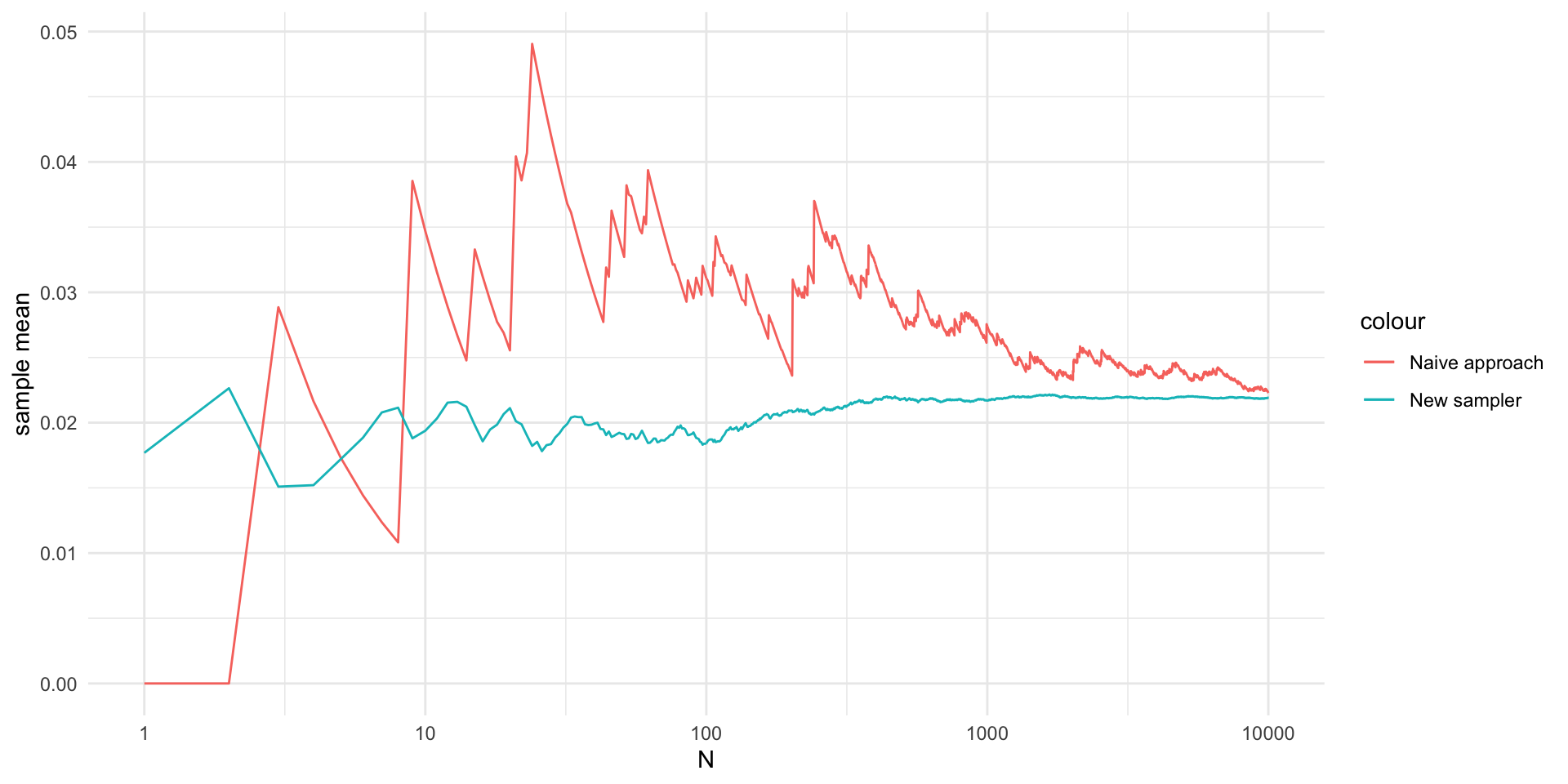
scale_x_continuous(trans='log10')Comparison
library(magrittr)
set.seed(2)
N = 10000
x = rnorm(N, 2, sqrt(1/2))

hnew = function(x) {
x[x < 1] = 0
x[x > 3] = 0
  return(x)
}

C = exp(-4) / sqrt(2)
# C = sqrt(1/2)

estimate = vector(length = N)
for (n in 1:N) {
  estimate[n] = mean(hnew(x[1:n]))
}

estimate = estimate*C

V2 = data.frame(x = seq(N),
               y = estimate)

V %>%
  ggplot(aes(x = x, y = y)) +
  geom_line(aes(color = "Naive approach")) +
  geom_line(data = V2, aes(x = x, y = y, col = "New sampler")) +
  theme_minimal() +
  labs(x = "N", y = "sample mean") +
  scale_x_continuous(trans='log10')