Covariance and Principal Components

Dr. Alexander Fisher

Duke University

Announcements

Reminder:

Final project presentations during lab Tuesday, April 25.

Covariance

Covariance and correlation

Empirical covariance between two variables

\[ cov(X,Y) = \frac{1}{n-1} \sum_{i = 1}^{n} (x_i - \bar{x})(y_i - \bar{y}) \]

Empirical correlation between two variables,

\[ \rho_{XY} = \frac{cov(X,Y)}{\sigma_X \sigma_Y} \]

where \(\sigma_X\) and \(\sigma_Y\) are the standard deviation of X and Y respectively.

Notice that the correlation matrix is just the covariance matrix of the standardized data.

Easy to see from definition of covariance

\[ cov(X, Y) = \mathbb{E} [(X - \mathbb{E}[X] ) (Y - \mathbb{E}[Y])] \]

`cov` and `cor` demo

x = c(1, 2, 3, 4, 5)
y = c(0.5, 3, 2.2, 5, 5.5)

demo
covariance matrix
correlation matrix

# covariance
cov(x, y)

[1] 3

# correlation
cor(x, y)

[1] 0.9243906

# covariance of standardized variables
xs = (x - mean(x)) / sd(x)# x-standardized
ys = (y - mean(y)) / sd(y)# y-standardized

cov(xs, ys)

[1] 0.9243906

d = data.frame(x = x, y = y)
cov(d)

    x     y
x 2.5 3.000
y 3.0 4.213

d = data.frame(x = x, y = y)
cor(d)

          x         y
x 1.0000000 0.9243906
y 0.9243906 1.0000000

Data

Hawks is a subset of a data set by the same name in the Stat2Data package. Today we will focus on the following measurements of 891 hawks:

Species: CH = cooper’s, RT = red-tailed, SS = sharp-shinned
Weight: body weight in grams
Wing: length in mm of primary wing feather from tip to wrist it attaches to
Culmen: length in mm of the upper bill from the tip to where it bumps into the fleshy part of the bird
Hallux: length in mm of the killing talon

Hawks = read_csv("https://sta101-fa22.netlify.app/static/appex/data/Hawks.csv")

glimpse(Hawks)

Rows: 891
Columns: 5
$ Species <chr> "RT", "RT", "CH", "SS", "RT", "RT", "RT", "RT", "RT", "RT", "R…
$ Weight  <dbl> 920, 990, 470, 170, 1090, 960, 855, 1210, 1120, 1010, 1010, 11…
$ Wing    <dbl> 385, 381, 265, 205, 412, 370, 375, 412, 405, 393, 371, 390, 41…
$ Culmen  <dbl> 25.7, 26.7, 18.7, 12.5, 28.5, 25.3, 27.2, 29.3, 26.0, 26.3, 25…
$ Hallux  <dbl> 30.1, 31.3, 23.5, 14.3, 32.2, 30.1, 30.0, 31.3, 30.2, 30.8, 29…

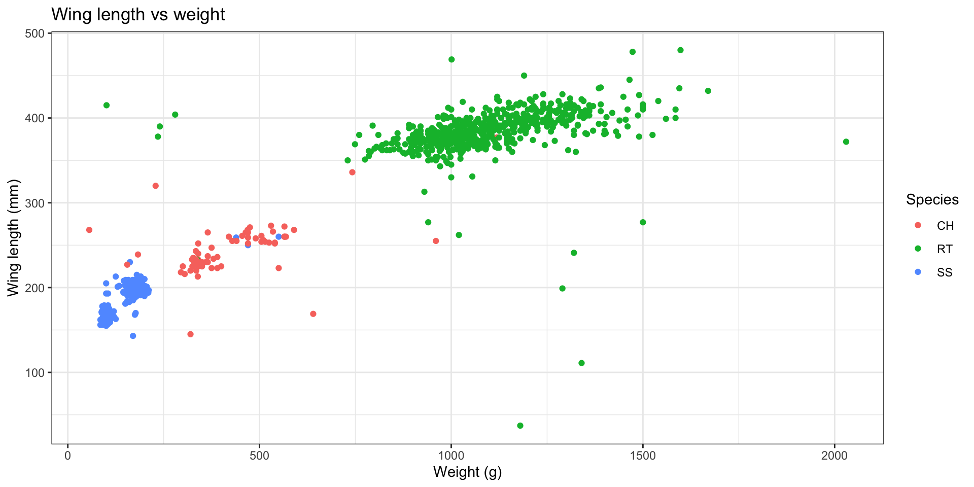
Visualizing covariance

Let’s look at hawk weight and wing length.

Data
Covariance matrix
Visualize covariance

# Covariance matrix
covMatrix1 = Hawks %>%
  select(Weight, Wing) %>%
  cov()

covMatrix1

          Weight      Wing
Weight 214310.57 41247.975
Wing    41247.97  9085.273

The mathematics of the covariance ellipsoid

Covariance matrix \(\Sigma\) collects variances and covariances together,

\[ \Sigma = \begin{pmatrix}\sigma_x^2 & \sigma_{xy}^2\\\ \sigma_{xy}^2 & \sigma_y^2\end{pmatrix} \]

How can we visualize the covariance matrix above?

The “matrix inverse” helps. The inverse of \(\Sigma\) is denoted \(\Sigma^{-1}\). The property of the inverse is:

\[ \Sigma^{-1} \Sigma = \begin{pmatrix}1 & 0\\\ 0 & 1 \end{pmatrix} \]

We can visualize the covariance matrix by forming the quadratic,

\[ z^T \Sigma^{-1} z = c^2, \]

where \(z = (x, y)\) and \(\Sigma^{-1} = \begin{pmatrix}s_x^2 & s_{xy}^2\\\ s_{xy}^2 & s_y^2\end{pmatrix}\). Where have we seen this before? Hint: see multivariate normal

Notice the linear equations

By multiplying out the product in scalar notation

\[ \begin{pmatrix} x & y\end{pmatrix} \begin{pmatrix}s_x^2 & s_{xy}^2\\\ s_{xy}^2 & s_y^2\end{pmatrix} \begin{pmatrix} x\\\ y \end{pmatrix} = c^2 \]

\[ (x s_x^2 + y s_{xy}^2 \ \ \ \ x s_{xy}^2 + y s_y^2) \begin{pmatrix} x\\\ y \end{pmatrix} = c^2 \]

\[ x^2 s_x^2 + 2x y \cdot s_{xy}^2 + y^2 s_y^2 = c^2 \]

This is the equation of an ellipse where our choice of \(c\) defines the size of the ellipse.

library(mvtnorm)
set.seed(1)

mu = c(5, 10)
sigma = matrix(data = c(2, .8, .8, 1), ncol = 2, nrow = 2)

points = rmvnorm(n = 500,
        mean = mu,
        sigma = sigma)

d = tibble(x = points[,1],
           y = points[,2]) 

d %>%
  head(n = 5)

# A tibble: 5 × 2
      x     y
  <dbl> <dbl>
1  4.20  9.96
2  4.41 11.2 
3  5.17  9.34
4  5.92 10.9 
5  5.68  9.91

ellipsePoints = data.frame(ellipse(sigma))
ellipsePoints["x"] = ellipsePoints["x"] + mu[1]
ellipsePoints["y"] = ellipsePoints["y"] + mu[2]

d %>%
  ggplot(aes(x = x, y = y)) + 
  geom_point() +
  theme_bw() +
  geom_path(aes(x = x, y = y), data = ellipsePoints,
             color = 'steelblue')

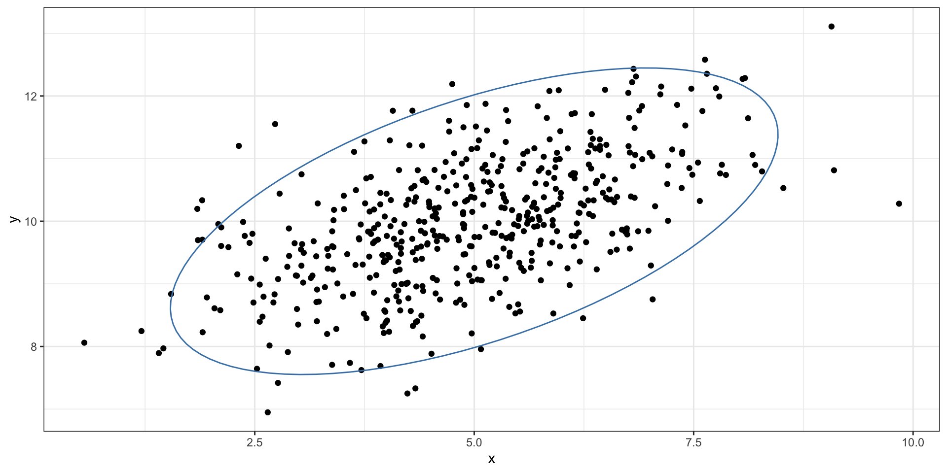
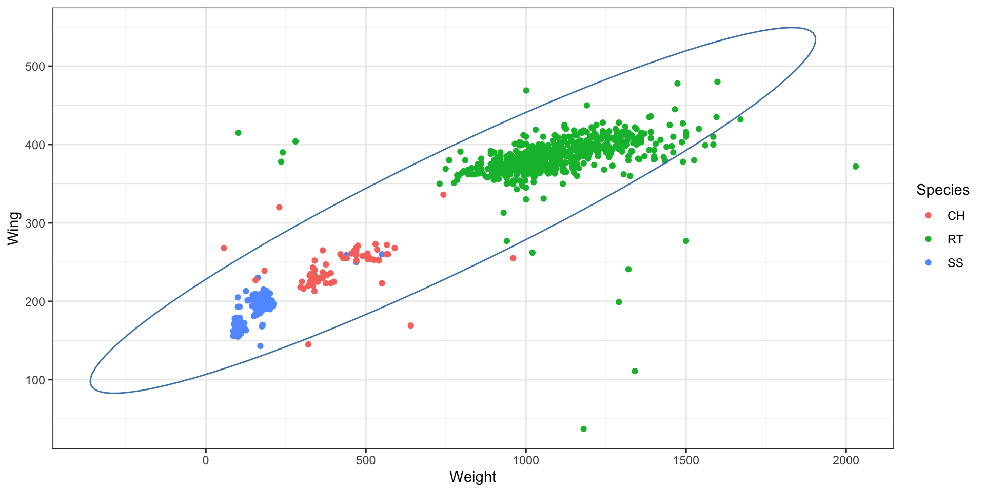
What \(c\) was used?

?ellipse has the answer… \(c^2 \approx 6\) for 2-d variables.

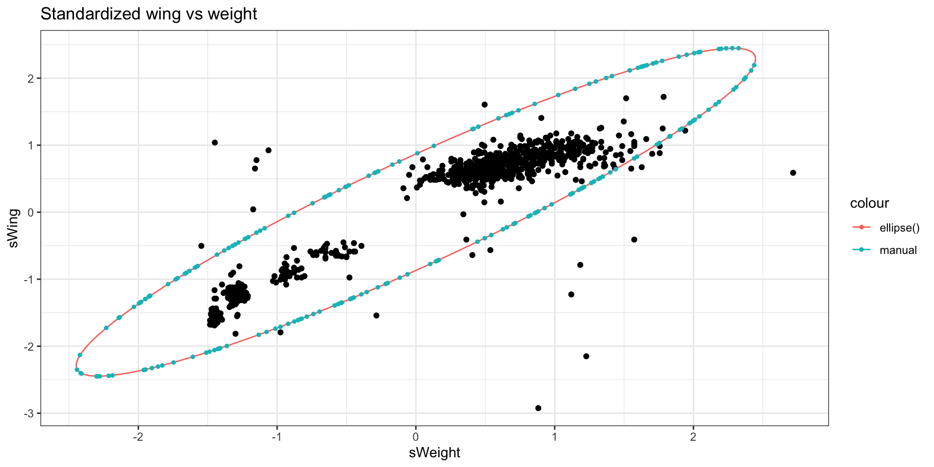
qchisq(0.95, 2)

[1] 5.991465

Exercise

prompt
1 - standardize
2 - solve quadratic
3 - plot comparison
4 - plot code

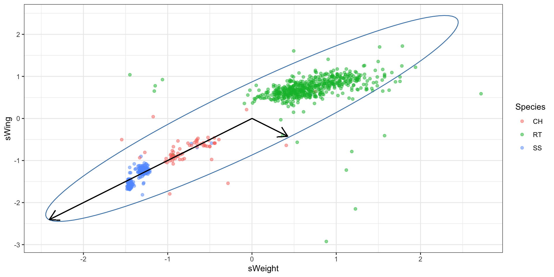
Perform a sanity check. Plot the ellipse manually using the formula from a previous slide and using \(c^2\) = 6. To avoid having to re-center on the centroid, you can standardize the data.

Hawks2 = Hawks %>%
  mutate(sWeight = (Weight - mean(Weight)) / sd(Weight),
         sWing = (Wing - mean(Wing)) / sd(Wing))

covMatrix2 = Hawks2 %>%
  select(sWeight, sWing) %>%
  cov()

covMatrix2

          sWeight     sWing
sWeight 1.0000000 0.9347852
sWing   0.9347852 1.0000000

Next, get \(\Sigma^{-1}\):

solve(covMatrix2)

          sWeight     sWing
sWeight  7.925401 -7.408548
sWing   -7.408548  7.925401

Next, we manually solve the quadratic equation using the quadratic formula (set \(c^2 = 6\))

\[ x^2 s_x^2 + 2x y \cdot s_{xy}^2 + y^2 s_y^2 = 6 \]

sx = 7.925401
sxy = -7.408548
sy = 7.925401

f = function(x) {
  A = sy 
  B = 2 * x * sxy
  C = (x * x * sx) - 6

  (-B + sqrt(B^2 - (4* A * C))) / (2 * A)
}

f2 = function(x) {
  A = sy 
  B = 2 * x * sxy
  C = (x * x * sx) - 6

  (-B - sqrt(B^2 - (4* A * C))) / (2 * A)
}

set.seed(1)
# Grab the points (x,y) that satisfy the equation
ellipsePoints = data.frame(ellipse(covMatrix2))
m1 = data.frame(x = seq(-3, 3, by = 0.001)) %>%
  mutate(y = f(x)) %>%
  filter(!is.nan(y))

m2 = m1 %>%
  mutate(y = f2(x)) %>%
  filter(!is.nan(y))

manualEllipsePoints = rbind(m1, m2) %>%
  slice_sample(n = 200)

Hawks2 %>%
  ggplot(aes(x = sWeight, y = sWing)) +
  geom_point() +
  theme_bw() +
  geom_path(aes(x = sWeight, y = sWing,
                 color = "ellipse()"), data = ellipsePoints) +
  geom_point(aes(x = x, y = y, color = "manual"), 
            data = manualEllipsePoints, alpha = 1,
            size = 1,) +
  labs(title = "Standardized wing vs weight")

Principal components

The axes of the ellipse provide the most informative directions to measure the data. In \(n\)-dimensions, where we have a \(n\)-dimensional ellipsoid, it can be useful to look at \(p<n\) axes. The largest axis is called the “first” principal component. The second largest axis is called the “second” principal component and so on.

Compute principal components

compute
plot
code

# get PCs
Hawks %>%
  select(Weight, Wing) %>%
  prcomp(scale = TRUE)

Standard deviations (1, .., p=2):
[1] 1.3909656 0.2553718

Rotation (n x k) = (2 x 2):
              PC1        PC2
Weight -0.7071068  0.7071068
Wing   -0.7071068 -0.7071068

# make plot
Hawks %>%
    mutate(pc1 = (0.7071068 * Weight) + (0.7071068 * Wing)) %>%
    ggplot(aes(x = pc1, y = 0, color = Species)) + 
    geom_point()

PCA summary

“Principal components” refers to the ranked orthogonal axes of the ellipsoid generated from the covariance matrix of the data.
The components are ranked largest to smallest.
PCA is a dimension-reduction technique. Often we examine the first 1 to 3 principal components to create visualizations of high-dimensional data.
What we gain in simplicity we often lose in interpretability. The ‘dimensions’ that capture the maximum variability of the data are created from linear combinations of the variables. These linear combinations are often difficult to interpret / motivate.

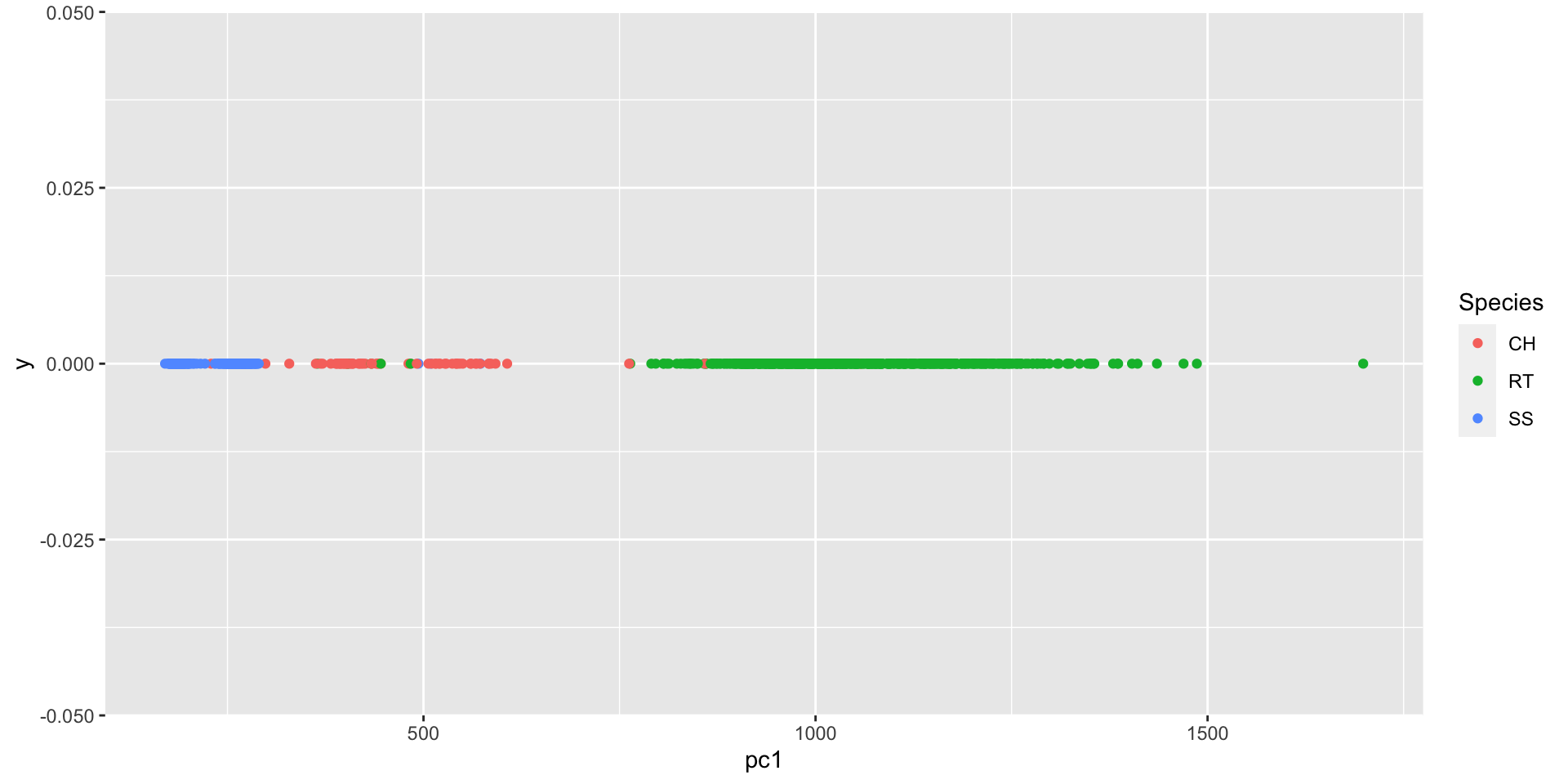
Higher dimensional example

plot
code

hpc = Hawks %>%
  select(Weight, Wing, Culmen, Hallux) %>%
  prcomp(scale = FALSE) %>%
  .["rotation"] %>%
  as.data.frame() %>%
  setNames(., paste0("PC", seq(4)))

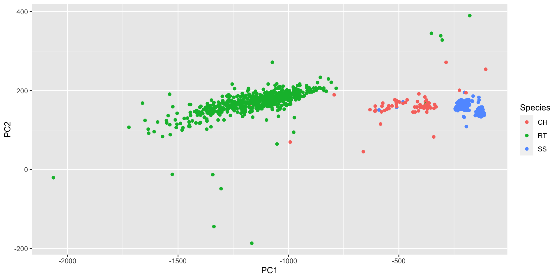
# explicitly mapping
Hawks %>%
  mutate(PC1 = (hpc$PC1[1] * Weight) + 
           (hpc$PC1[2] * Wing) + 
           (hpc$PC1[3] * Culmen) + 
           (hpc$PC1[4] * Hallux),
         PC2 = (hpc$PC2[1] * Weight) + 
           (hpc$PC2[2] * Wing) + 
           (hpc$PC2[3] * Culmen) + 
           (hpc$PC2[4] * Hallux)) %>%
  ggplot(aes(x = PC1, y = PC2, color = Species)) +
  geom_point()

Covariance and Principal Components

Announcements

Covariance

Covariance and correlation

cov and cor demo

Data

Visualizing covariance

The mathematics of the covariance ellipsoid

Notice the linear equations

Connection: MVN

Exercise

Principal components

Principal components

Compute principal components

PCA summary

Higher dimensional example

Further reading

`cov` and `cor` demo